This is series of blog posts of me trying to share what I’ve explored in the course ‘From Deep learning foundations to Stable Diffusion’ by FastAI.
The things I am about to share in this post is based on the initial lessons of the course, which is publicly available here. The lessons also have some accompanying jupyter notebooks on stable diffusion, which can be found in this Github repo.
Let’s jump right into the post with the question: ‘What is stable diffusion?’.
What is stable diffusion?
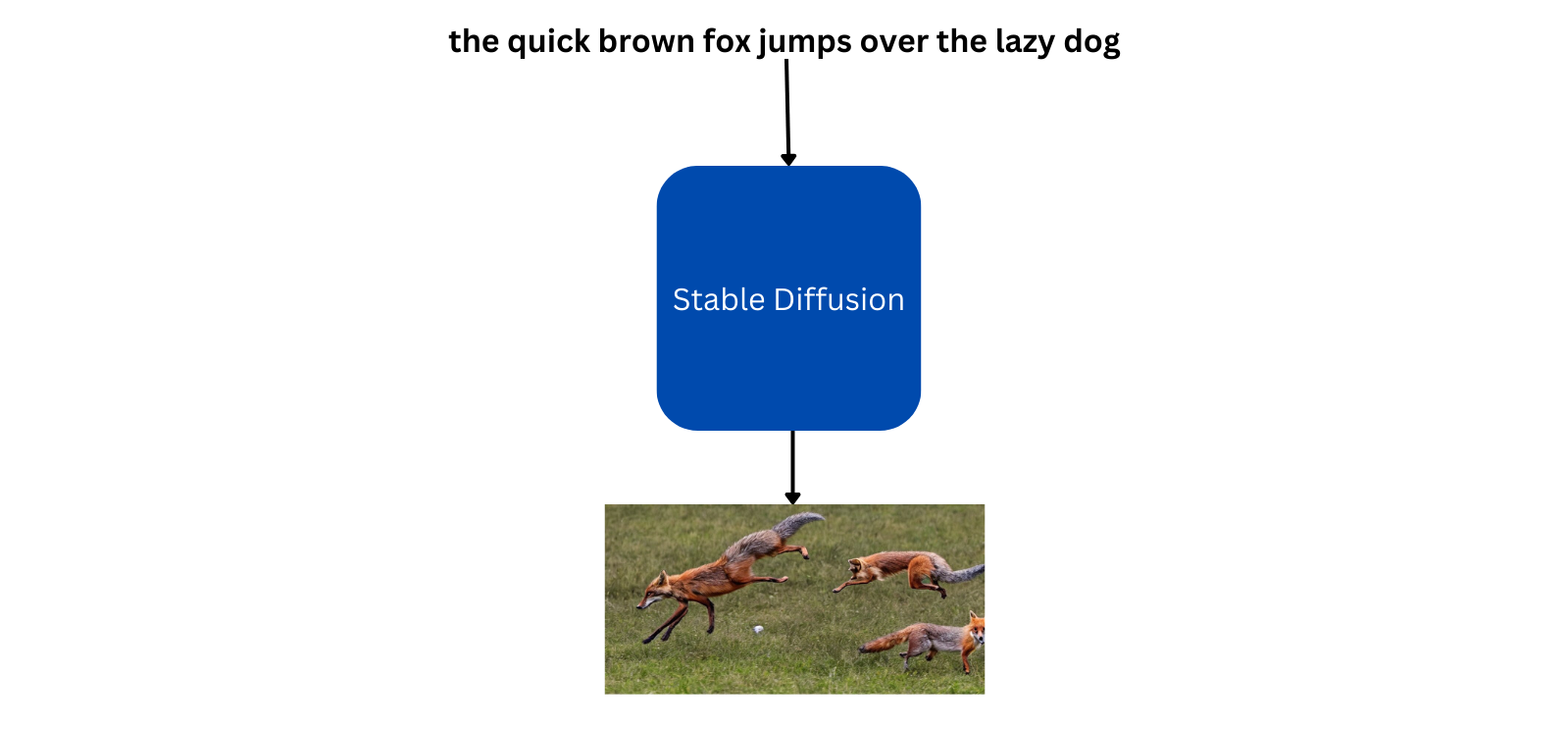
In simple words, stable diffusion is a deep learning model that can generate an image given a prompt like below:
It can also take an image as a starting point along with a prompt, to generate an image similar to the input image.For example, if the model is given a random drawing of wolf looking at the moon along with the prompt ‘wolf howling at the moon’, the model will generate a good looking image with similar setting as the input image:

But how does this whole thing work?
First, let’s see how the model generated an awesome wolf image from a random sketch and a simple prompt. This generation process involves 3 different models:
- A model for converting the text prompt to embeddings. Openai’s CLIP(Contrastive Language-Image Pretraining) model is used for this purpose.
- A model for compressing the input image to a smaller dimension(this reduces the compute requirement for image generation). A Variational Autoencoder(VAE) model is used for this task.
- The last model generates the required image according to the prompt and input image. A U-Net model is used for this process.
We will summarize each of the process above using simple diagrams:
CLIP Embeddings
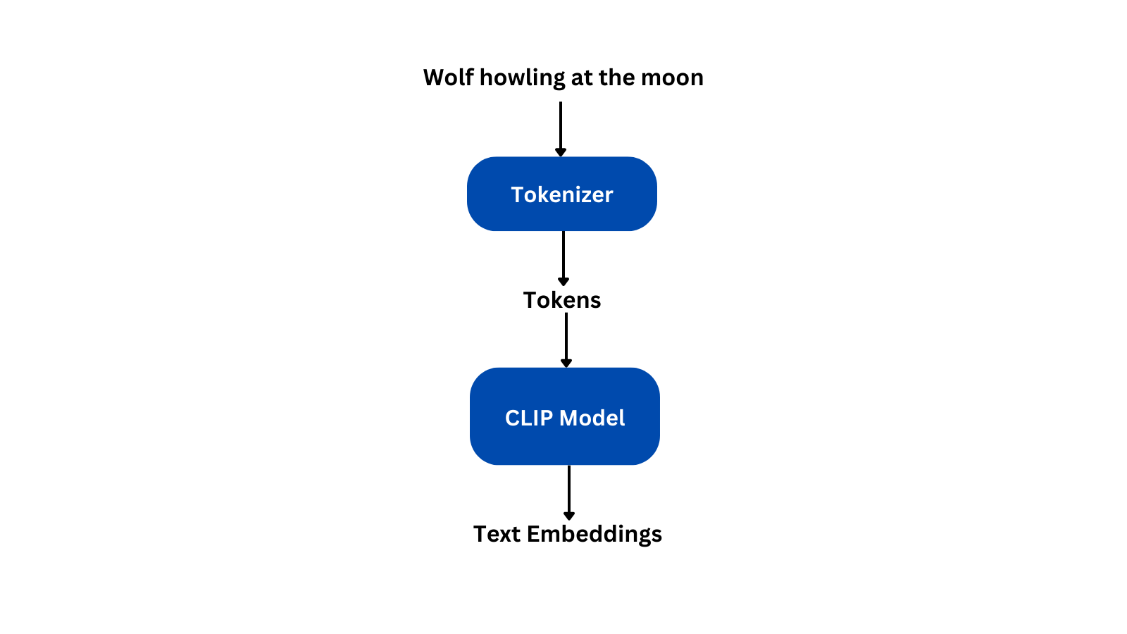
As seen from the above figure, the prompt is converted to tokens using a tokenizer and these tokens are fed into the CLIP model to get the final text embeddings.
Encoder part of VAE model
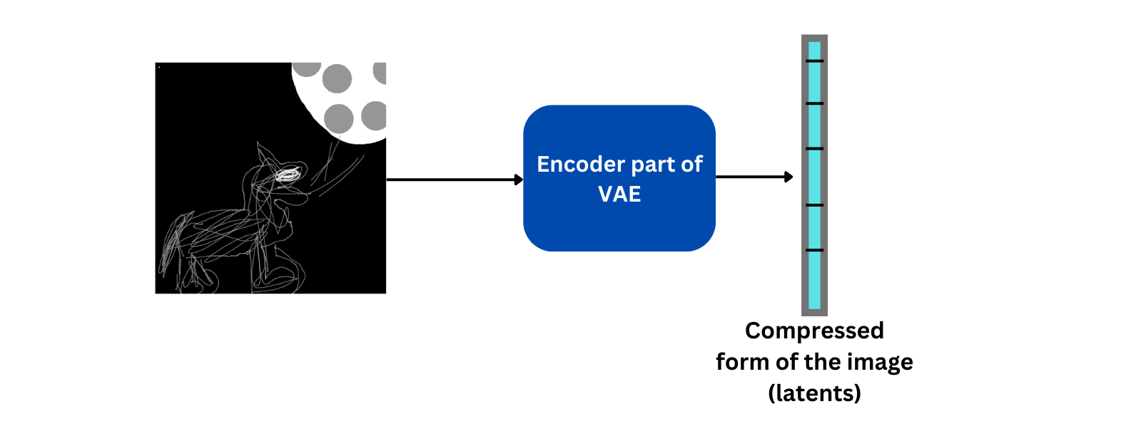
The VAE model has an encoder as well as a decoder part. Given an image, the encoder part of the VAE compress the image to a low dimension tensor without much loss in information. This compressed form is called latents. The decoder is used to recover the original image from the latents. In the figure above only the encoder part is shown, we will talk more about decoder in the coming steps.
U-Net model
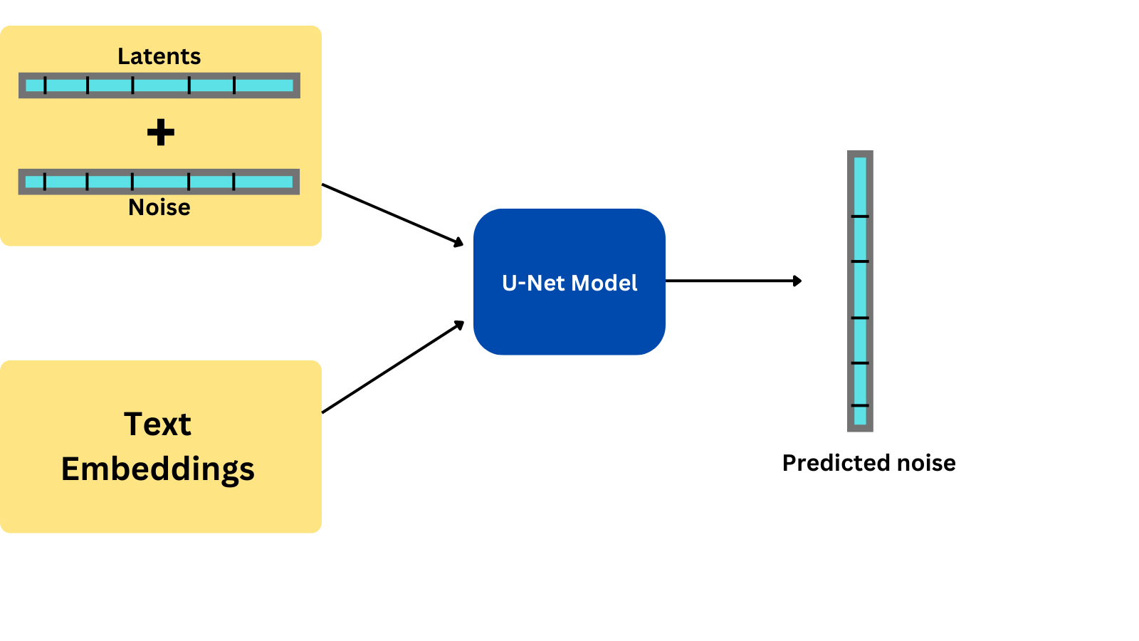
The U-Net model takes in the latents created by VAE as well as the text embedding created by the CLIP model as inputs. But before we pass in the latents, we add some noise to it, so that the U-Net model does not completely copy the image as it is.
With the noisy latents combined with text embeddings as inputs, the U-Net model tries to predict the noise present in the latents. We subtract this predicted noise from the latents to get the original latents. We repeat this process a specified number of times, say for example, 50 times. During each iteration, the amount of noise added to the latents is reduced.
So we start with a very noisy latent and gradually reduce the noise added.
Once the specified number of iterations is over, we get some latents that is ready to be decoded to an image. For this, we use the decoder part of the VAE model as shown below:
Decoder part of VAE model
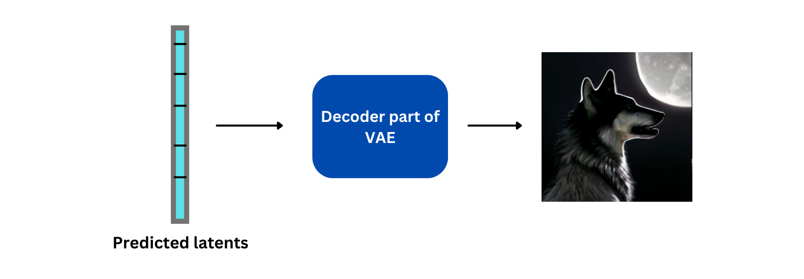
This is simplified version of how stable diffusion model generates an image given a prompt and an initial image. Since these models work on latent space rather than the original image, these types of models are also called latent diffusion models.
As said earlier in the post, stable diffusion model can generate image even if we only provide a prompt describing the image we want. The above pipeline remains the same for this task also, but the only difference is that we don’t require the encoder part of the VAE model as we dont have any initial images to encode. So we just create a random tensor with the same size as the latents to feed to out U-Net model.
Looking into the source code of huggingface diffusers
Playing around with diffusers
The diffusers library from huggingface already has implementations of the stable diffusion model and the library makes it easier to play around with these types of models.
Before you can play around with these models, you need to go here and accept the terms and conditions. Once you do that, you need to create a new token from here and copy it into the box that appears when you run the follwoing code in your jupyter notebook:
!pip install huggingface-hub==0.10.1

from huggingface_hub import notebook_login
notebook_login()
Once everything is completed successfully, install the dependencies(as of writing this post, the latest version of diffusers and transformers are 0.6.0 and 4.23.1 respectively):
!pip install -qq -U diffusers transformers
Generating images with diffusers and stable diffusion is as simple as running these 3 lines of code(the code requires a GPU machine):
from diffusers import StableDiffusionPipeline

# set up the pipeline to generate images
pipe = StableDiffusionPipeline.from_pretrained(
    'CompVis/stable-diffusion-v1-4',
).to('cuda')

prompt = "a photograph of an astronaut riding a horse"
# generate an image for the above prompt
pipe(prompt).images[0]
If you wish to play around with diffusers pipeline for image generation, do check out their documentation here.
Diving deeper into StableDiffusionPipeline
Now let’s look into the source code and see what exactly is going on when we pass the prompt to our pipeline. The exact code that I’m discussing here can be found here.
First, let’s learn more about the arguments in our pipeline:
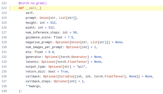
Other than the prompt we pass, there are a bunch of other arguments too. We can customize the image generation process by changing the default value of these arguments.
Let’s check each of the arguments:
prompt- this is the prompt that we pass to our pipeline as inpipe(prompt).height,width- these are the dimensions of the generated image.num_inference_steps- as we’ve discussed before, the unet model runs multiple times before generating the final latents, this argument defines this number.guidance_scale- guidance scale is the value that decides how close should our image be to the prompt. This is related to technique called Classifier-Free Guidance(CFD).negative_prompt- this is another argument that takes in a prompt as input. But as the name suggests, this is a negative prompt, thus, the model will try to generate images that doesn’t have any similarities with this prompt. As an example, if we provide ‘blue color’ as a negative prompt, the model will try to avoid including the color blue in the generated image.num_images_per_prompt- the number of images to generate for a given prompt.callback- this is mostly a callable function, that allows you to add some custom code into the pipeline.callback_steps- number of times the callback function will be called.
The documentation page of diffusers has all these arguments listed with details included.
Now let’s move to the improtant parts of the pipeline. The code below shows the text encoding part of the model:
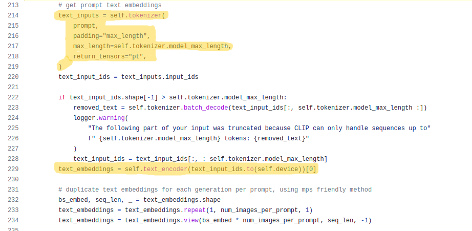
The first highlighted part shows the code for tokenizing our prompts using a tokenizer, pads it to the maximum length of the model and returns the tokens as pytorch tensors. The second highlighted part is where we pass these tokens to the CLIP model(text_encoder in the code) and gets the text embeddings.
The below code sets everything for classifier-free guidance we talked earlier:
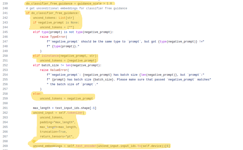
Classifier free guidance is done only if the guidance scale is greater than 1, the first highlighted part(line 239) checks this condition.
For doing classifier guidance, we need a new prompt called unconditional prompt which is an empty string(line 244) if no value is passed to negative_prompt, otherwise, the same negative prompt is used as unconditional prompt(line 251 & line 259).
After deciding on the unconditional prompt, the prompts are tokenized(line 262) in the same manner as the normal prompts and encoded using the CLIP model(line 269).
Once we are ready with the unconditional embedding and the text embedding, we concatenate them and move on to the next step:
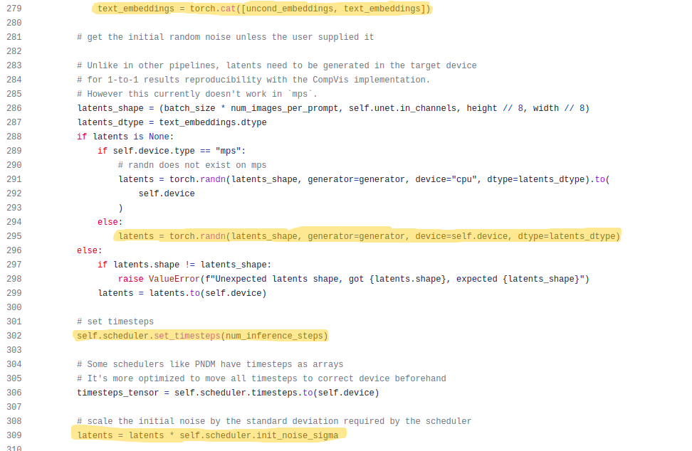
The concatenation part is done in the first highlighted part. Once we have the embedding part of our input ready, we need to prepare the second input, that is the latents. For that we just create a random tensor(line 295) with the same shape as the latents created by our VAE model from an image.
We have a scheduler which decides the amount of noise to be added to the latent at each iteration, so we give it the information regarding the maximum number of iterations(shown in line 302).
As said earlier we add noise to the latents before passing it to the U-Net model(shown in line 309).
Everything is set, now it’s time to enter the generation step:
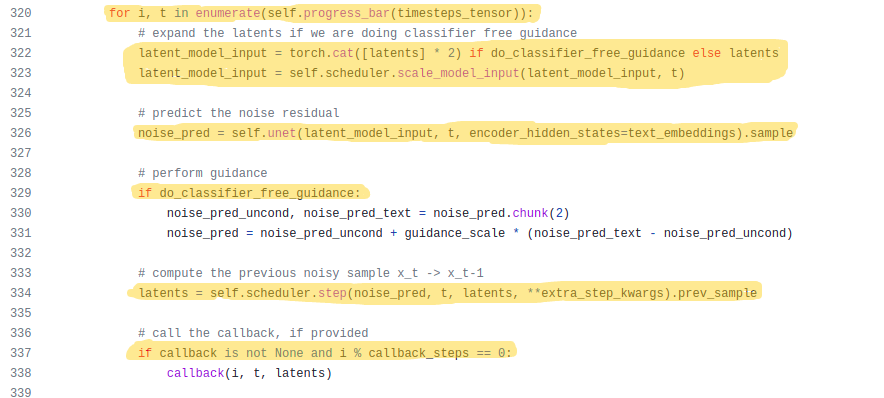
In the generation process, we iterate for the specified number of times(line 320). If we are doing classifier free guidance, we need to duplicate our latents(line 322) because we have an unconditional embedding and a text embedding. So in order to generate one image for each of these embeddings, we need separate latents for them.
In the next two lines of code, we scale the latents as required by the U-Net model and the model predicts the noise present in the input latents. Thus if we are doing classifier free guidance, the model will output two latents, otherwise, only one.
For classifier free guidance, we get the original noise to subtract from our latents from the follwoing formula(line 331):
predicted_noise = noise_predicted_for_unconditional_embedding + guidance_scale*(noise_predicted_for_text_embedding - noise_predicted_for_unconditional_embedding)
The above equation is where the guidance scale comes into play. It has a huge effect on the final noise subtracted from our latents.
Finally, we pass the generated noise and the current latents to our scheduler to add noise for the next iteration(line 334). One thing to note here is that
A new feature that was added recently is the callback function. If we pass any arguments to the callback argument, it gets executed inside the pipeline at line 338. For example, let’s create a simple function to pass into callback argument:
def sample_function(i, t, latents):
    # callback function expects the above 3 arguments
    print(i, t)
Now if we pass in this function to the pipeline as pipe(prompt, callback=sample_function, callback_steps=3), then the function will be executed 3 times and each time it will print the values of i and t.
At last, we’ve reached the end of this source code deep dive, this is where the latents are coverted to image tensor using the decoder part of VAE model and then returns as a PIL image(shown in the highlighted part below).
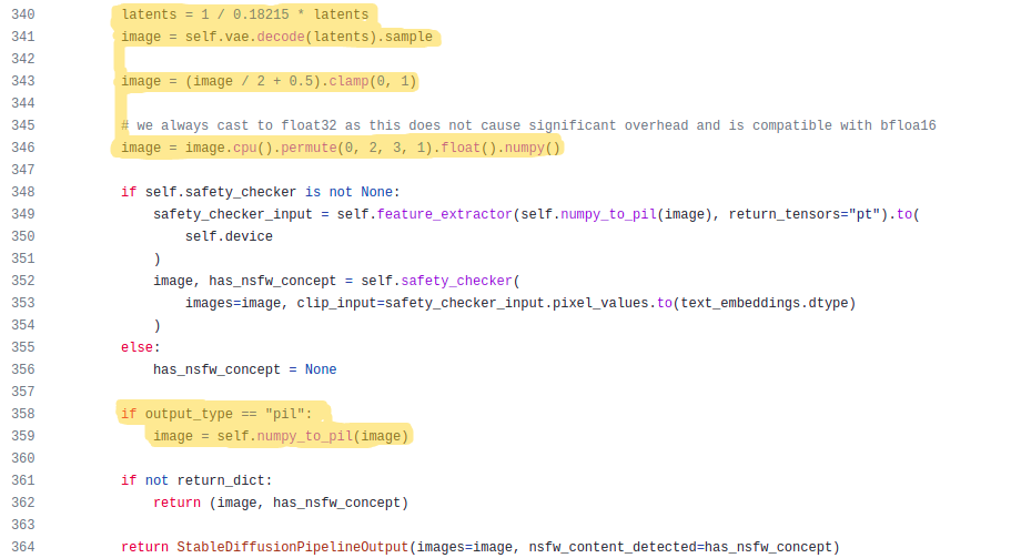
The code that is in between the highlighted part(line 348 to 356) is used for checking the generated image for NSFW(Not Safe For Work) content. If this type of content is detected, the pipeline returns a black image as of the current version of the library(v0.6.0).
Concluding thoughts
This is just an overview of what’s happening inside diffusion models and the stable diffusion pipeline in diffusers.
To get an in-depth explanation on the topic and learn some cool tricks with stable diffusion, you should definitely checkout the FastAI course lectures and accompanying notebooks listed at the top of this blog post. If you have any queries or want to discuss something machine learning, you could reach out to me via twitter @bkrish_.